Using CLP(FD) to solve factorial and fibonacci problems reversely
Running program backward in logic programming
One interesting features of logic programming languages like Prolog is that
it can run some programs backward, which means that given the output of the
program, it can yields all the input satisfies the relation. One famous example
is the append function of list.
my_append([], Ys, Ys).
my_append([X|Xs], Ys, [X|Zs]) :- my_append(Xs, Ys, Zs).
The above prolog program give the relation that my_append(Xs, Ys, Zs) which
means that list Xs append list Ys the result is list Zs. In a functional
languages, the append function is normally given two list and return the
result of the concatenation of them. But with automatic backtracking of logic
programming, we can actually call the relation with the output, and get all the
input. For example, the following is calling my_append(Xs, Ys, [1,2,3,4])
which means for what Xs and Ys, their concatenation is list [1,2,3,4].
?- my_append(Xs, Ys, [1,2,3,4]).
Xs = [],
Ys = [1, 2, 3, 4] ;
Xs = [1],
Ys = [2, 3, 4] ;
Xs = [1, 2],
Ys = [3, 4] ;
Xs = [1, 2, 3],
Ys = [4] ;
Xs = [1, 2, 3, 4],
Ys = [] ;
false.
We can see that the program automatically return us all the possible answer for
Xs and Ys whose concatenation is [1,2,3,4].
The magic behind the sceen is the automatica backtracking search of logic programming languages through unification algorithm which was first investigated by John Alan Robinson, so it is also called Robison Unification algorithm.
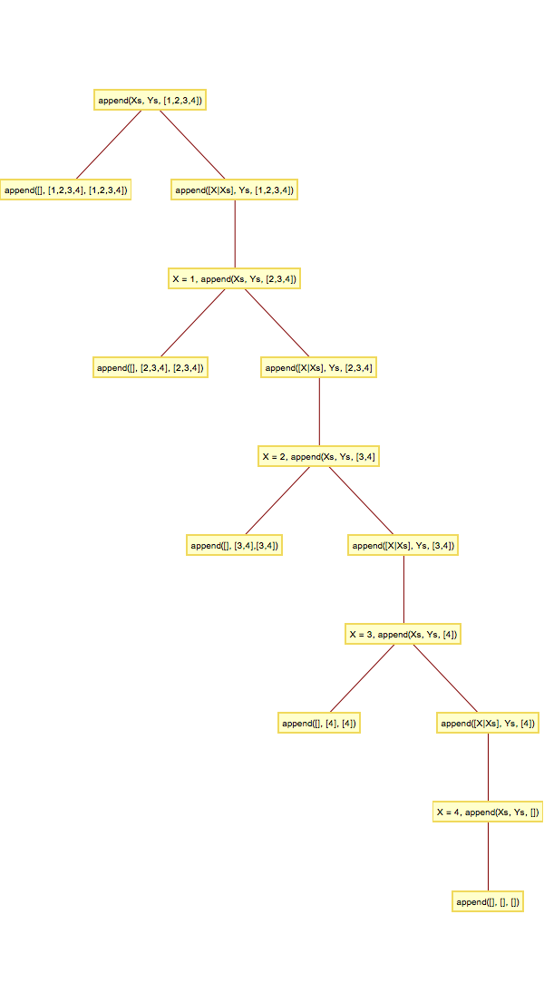
search tree of append
The above picture shows the search tree of the append, each leaf node is a
solution of my_append clauses. Notic in each intermediate node there are
two ways to do the unification for each of the my_append clause respectively.
Question about run factorial backward
Over the past few days, there are some people on Quora asked me how to
solve the problem of X! = N in prolog. Although prolog has the ability to
run program backward, sadly, logic programming can not be used directly in
this scenario since the program of fact as follow do use the value of
N in the body.
fact(0, 1).
fact(N, F) :-
    N >= 1, N1 is N - 1,
    fact(N1, F1),
    F is N * F1.
?- fact(5, F).
F = 120 ;
false.

?- fact(7, F).
F = 5040 ;
false.

?- fact(N, 120).
ERROR: >=/2: Arguments are not sufficiently instantiated
?-
The above example shows that when we call fact(N, 120), the prolog system
will complain that >= arguments are not sufficiently instantiated. It is
because that we actually use the value which is not given in the call.
Constraint programming to rescue
At first, I try to solve it in pure prolog. So I try to use a binary search algorithm to solve the problem. But late on, I remeber the constraint logic programming model I recently explored, so I decided to give it a try.
In short, constraint programming is a programming paradigm which is even more high level programming model than functional and logic programming. In this model, programmer just need to state the constrains the variable need to satisfy instead of writing the whole algorithm. The constraint solver will try to solve the problem automatically.
Based on the domain, constraint programming normally has the the following categories:
- Finite Domain : such as integers, set etc
- Real domain : such as linear optimization
- Boolean domain : deal with boolean value such as SAT
- Tree domain
Since the holistic discussion is beyond this post, readers who are interested in constraint programming are encourage to read Peter J. Stucky’s book “Programming with constrain: An introduction”.
Here I just show you how use “clp(fd)” library in swi-prolog to make a general relation of factorial in prolog.
:- use_module(library(clpfd)).

n_factorial(0, 1).
n_factorial(N, F) :-
    N #> 0, N1 #= N - 1, F #= N * F1,
    n_factorial(N1, F1).
Some calling example of n_factorial as follow:
?- n_factorial(5, F).
F = 120 ;
false.

?- n_factorial(10, F).
F = 3628800 ;
false.

?- n_factorial(N, 120).
N = 5 ;
false.

?- n_factorial(N, 720).
N = 6 ;
false.

?- n_factorial(N, 721).
false.
Facing the problem of non-termination
If you’re a scrupulous programmer, you will notice that the constraint version
has a difference with the normal version, it reverse the last two clauses at
last. It is done deliberately to avoid non-termination problem. If we reorder
the last two clause to the same order as in fact, we get the program as
follow:
:- use_module(library(clpfd)).

% non termination after reordering.
n_factorial2(0, 1).
n_factorial2(N, F) :-
    N #> 0, N1 #= N - 1,
    n_factorial2(N1, F1),
    F #= N * F1.
When we call n_factorial2(N, 120), after finding the first solution N = 5,
the program fall into a infinite search.
Constraint logic programming, same as its host logic programming languages, normally face the problem of divergence, which means it can lead to an infinite search if programmed without care.
At first, I am a little confused by the behavior of the non-termination. After ask for the help of clp(fd)’s author Markus Triska, various help I get from ##prolog irc channel and books, thesis on relation programming in miniKanren, I finally found out why.
The problem is although that system like clp(fd) and miniKanren is designed
with strong termination guarantees, they’re still using the principle that goal
appear first will also excute first, which means instead of doing the constraint
clause F #= N * F1, it will now first excute n_factorial2(N1, F1) which
finally diverges because there are infinite Ns which satisfy the constrains.
The short law that one program in logic/relational programming and constraint logic programming is that as stated in William E. Bryd’s disseration “unification should always come before recursive call, or calls to other serious relations”. For constraint logic programming, it is “constraint should always come before recursive call”.
Use constraint logic programming to solve fibonacci problem
This paradigm can be used to solve a wide range of relational programming on finite domain such as integers. So it is definitively can be applied to the fibonacci number problem.
Here is the fibonacci number problem in prolog.
n_fib1(0, 1).
n_fib1(1, 1).
n_fib1(N, F) :-
    N > 1, N1 is N - 1, N2 is N - 2,
    n_fib1(N1, F1),
    n_fib1(N2, F2),
    F is F1 + F2.
Sadly, translate the above program to clp(fd) does not produce a convergent program.
:- use_module(library(clpfd)).

% non termination due to infinite solution to constrain of F #= F1 + F2.
n_fib1(0, 1).
n_fib1(1, 1).
n_fib1(N, F) :-
    N #> 1, N1 #= N - 1, N2 #= N - 2,
    F #= F1 + F2,
    n_fib1(N1, F1), n_fib1(N2, F2).
The problem is clearly discussed in a excellent stackoverflow answer, in
short, the problem is caused by the fact constrain F #= F1 + F2 has infinite
solution, which will yield divergence. So the natural thought is that to add
constrain F #> 0 to the program. But this still does not work, since the
constraint F #= F1 + F2, F #> 0 still has unlimited solution.
The right way is as said in the stackoverflow answer, add the constriants
F1 #> 0, F2 #> 0, be aware also to follow the law to do relational/logic
programming and constraint programming, make them before the recursive call.
So the final work solution is as follow:
:- use_module(library(clpfd)).

% terminate add constrains of F1 #> 0, F2 #> 0.
n_fib4(0, 1).
n_fib4(1, 1).
n_fib4(N, F) :-
    N #> 1, N1 #= N - 1, N2 #= N - 2,
    F #= F1 + F2, F1 #> 0, F2 #> 0,
    n_fib4(N1, F1), n_fib4(N2, F2).

?- n_fib4(N, 8).
N = 5 ;
false.

?- n_fib4(N, 13).
N = 6 ;
false.

?- n_fib4(N, 15).
false.
But the above problem has efficiency problem since naive fibonacci algorithm runs in exponent time complexity. This can be showed from the running time in prolog.
?- time(n_fib4(N, 55)).
% 196,914 inferences, 0.036 CPU in 0.036 seconds (100% CPU, 5402819 Lips)
N = 9 ;
% 6,662,749 inferences, 1.319 CPU in 1.463 seconds (90% CPU, 5051567 Lips)
false.
We can see when call n_fib4(N, 55) it will yield the first answer in around
0.04s, and will finish search for other answer in around 1.3s. If this is the
case, then it will definitively not be able to solve large problems.
Use same idea in functional programming to accelerate n_fib4
In functional programming, we can add another argument to make it a dynamic like algorithm for fibonacci number, so that it can run in linear time as the following code in haskell
fib n = go n 0 1
    where
    go n a b | n==0 = a
             | otherwise = go (n-1) b (a+b)
We can use the same idea in constraint logic programming here.
:- use_module(library(clpfd)).

% accerlate n_fib4
n_fib6(0, 1, 0).
n_fib6(1, 1, 1).
n_fib6(N, F, F1) :-
    N #> 1, N1 #= N - 1,
    F #= F1 + F2,
    F1 #> 0, F2 #> 0,
    n_fib6(N1, F1, F2).
Now we can call the following example and it’s much much faster than the naive recursive version.
?- time(n_fib6(N, 377, F2)).
% 77,602 inferences, 0.014 CPU in 0.014 seconds (100% CPU, 5468345 Lips)
N = 13,
F2 = 233 ;
% 868 inferences, 0.000 CPU in 0.000 seconds (99% CPU, 2376832 Lips)
false.

?- time(n_fib6(N, 378, F2)).
% 80,399 inferences, 0.015 CPU in 0.015 seconds (100% CPU, 5325256 Lips)
false.
Conclusion
Constraint programming is a really undervalued programming paradigm which is ignored by most people. But we should also notice that there is no free meal either, we should be very careful to add additional constrains as in the above example showed, but it is still a very very powerful paradigm for general relational programming which deserve to be known. It will extremely broaden one’s view of programming in general. You could find the whole experiment program from miscellaneous-code/fact-and-fib-in-clpfd.
m00nlight 01 January 2016